
We illustrate the uncertainty around our forecasts using a variety of approaches. This box described using stochastic simulations to produce fan charts, which could be used to enhance presentation of uncertainty in future EFOs, and showed some experimental results.
This box is based on OBR data from October 2021 .
We currently illustrate the uncertainty around our central forecasts using a combination of: (i) probabilistic fan charts based on historical forecast errors for key macroeconomic and fiscal
aggregates; (ii) sensitivity analysis, which looks at the fiscal implications of shocks to individual forecast determinants; and (iii) scenarios that explore the fiscal implications of a plausible combination of shocks to multiple forecast determinants. All this analysis is informed by our annual Forecast evaluation report, which looks at the scale and sources of our economic and fiscal forecast errors, and identifies lessons for future forecasts.
To enhance the presentation of uncertainty in future EFOs, we have been investigating the use of stochastic simulations to generate fan charts. The approach works by generating a very large
number (thousands) of scenarios that are each driven by randomly selected shocks that are typical of those that have been experienced in the past. The output can then be used to evaluate metrics of interest, such as the proportion of the scenarios in which some target criterion is satisfied. This approach is widely used in the academic literature and by other organisations, including by the IMF in its ‘Article IV’ assessments of countries’ public debt sustainability.a
Using stochastic simulations has several advantages over using historical forecast errors. These include allowing us to capture a longer, and perhaps therefore more representative, history of shocks that have hit the UK economy, or to calibrate against particular sub-periods, such as the particularly benign period running from 1993 to 2006 (the ‘Great Moderation’). The approach ensures greater consistency between fan charts for different variables. It also allows us to produce a fan chart for the level of PSND as it captures the persistence and skew in debt. Finally, it allows us to assess the probability of meeting different types of target more easily, and facilitates the calculation of the probability of meeting more than one target at the same time.
We start by estimating a small vector autoregression (VAR) model that captures the dynamic interrelationships between real GDP, inflation, interest rates, and the primary balance, to which we append the public sector budget identity that relates public sector debt to these variables. The model therefore incorporates an average historical response of both fiscal and monetary policies to economic developments, as well as the impact of those policies on the economy.
This structure can then be used to trace through the consequences of a shock to, say, GDP or inflation. However, rather than draw these shocks from some normal distribution, informed by historical forecast errors we draw our shocks from the vectors of historical residuals in the VAR (the estimated equations of the VAR do not fit exactly, leaving an unexplained ‘residual’). Consequently, our simulations match the historical distribution of the residuals, including any skewness and ‘fat tails’, as well as replicating the empirical correlations between them.
For each period of each simulation, we draw the shocks from a suitable sample period; in the example here that extends from the mid-1950s to the present. We can, though, vary the sample period from which shocks are chosen; for example, a period spanning the ‘Great Moderation’ would produce much narrower fans, while one running from the financial crisis to the pandemic and including both would produce wider ones. We then repeat this process several thousand times, allowing us to generate probability distributions for each of the variables.
As a final step, we align the median of the distributions from the stochastic simulations with our central forecast that embodies our own forecast judgements and explicitly factors in current stated policies. This means that the central forecast reflects our own judgements, while the size and shape of the uncertainty fan around it is determined by the long run of history captured in the VAR. We will publish further detail on the methodology in a forthcoming discussion paper.
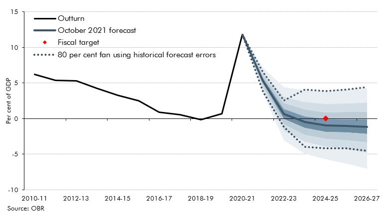
Chart A shows some initial experimental results from the analysis for public sector net debt (excluding the Bank of England). The centre of the fan (our central forecast) is the median, meaning there is a 50 per cent chance of debt being above or below it. Each of the four bands on each side of the median represents 10 percentage points within the overall probability distribution, implying an 80 per cent chance that debt will be within the fan in each year. So for example, in the fiscal target year of 2024-25 there is a 20 per cent chance that debt will be between 80 and 90 per cent of GDP and an 80 per cent chance that it will be between 60 and 118 of GDP. The width of the fan increases over time, with the 80 per cent interval widening from 26 per cent of GDP in 2022-23 to 92 per cent of GDP in 2026-27. A similar pattern can be seen in the case of the fan around the current budget deficit forecast (Chart B).
The fans generated by this approach are somewhat wider than those based on historical forecast errors, particularly in the near term. The current budget balance fan has less of a negative skew in this approach, reflecting the inclusion of pre-1980 shocks, most notably the unanticipated very high levels of inflation experienced in the 1970s. But the two approaches both produce fans with similar upward skews for changes in PSND, as the simulation approach captures ‘stock-flow adjustments’ (changes in debt that are not from borrowing, such as net acquisition of financial assets) that have historically had an upward skew.
Chart A: Fan chart around PSND forecast excluding Bank of England
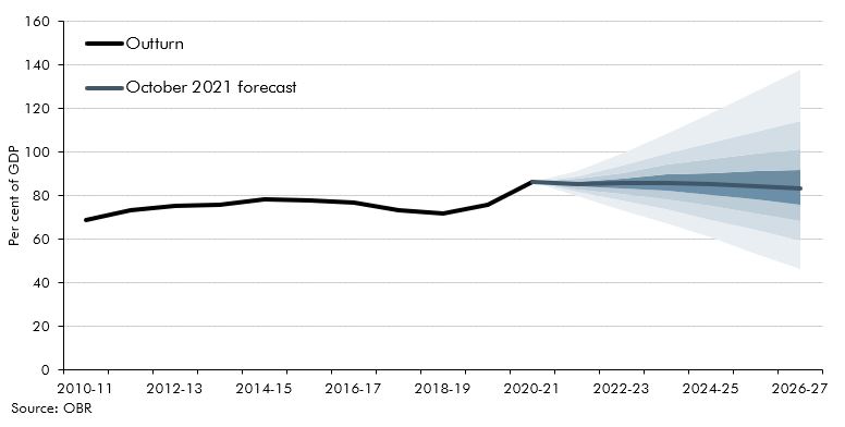
Chart B: Fan chart around current budget deficit
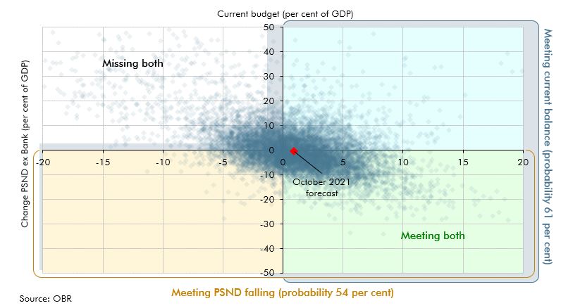
The simulations underpinning these fan charts can also be used to produce an assessment of the probability of meeting the new fiscal targets. To assess the probability of debt falling in 2024-25, we can calculate the fraction of simulations in which debt falls in that year. This suggests a 54 per cent chance of debt falling and the fiscal mandate being met. For the current budget balance target in 2024-25 the probability is 61 per cent.
We can also use the simulations to show the combined probability of meeting both of these targets in 2024-25 (the fraction of simulations where debt falls as a share of GDP and the current budget is in balance). Chart C shows a scatter plot of the different simulation values for the current budget and change in debt in 2024-25, where the darker the area the more simulations point to that outcome. The bottom two quadrants show where PSND is falling (in 54 per cent of simulations), the two quadrants on the right show the current budget in surplus (61 per cent of simulations), while the bottom right quadrant shows where both targets are met at the same time (just 40 per cent of simulations). This shows that while both targets are met in our central forecast (the red diamond), on average across all the simulated futures there are more occasions where one or both targets are missed than there are where both are met.
Chart C: 10,000 simulations of current balance and change in PSND in 2024-25
This box was originally published in Economic and fiscal outlook – October 2021